Decoding with Sorted Spikes#
import logging
import os

import matplotlib
import seaborn as sns
import numpy as np
import matplotlib.pyplot as plt

# Make analysis reproducible
np.random.seed(0)

# Enable logging
logging.basicConfig(level=logging.INFO)
Create Simulated Data#
from replay_trajectory_classification.sorted_spikes_simulation import make_simulated_run_data

time, position, sampling_frequency, spikes, place_fields = make_simulated_run_data()
WARNING:replay_trajectory_classification.core:Cupy is not installed or GPU is not detected. Ignore this message if not using GPU
Plot the spikes and the position:
MM_TO_INCHES = 1.0 / 25.4
ONE_COLUMN = 89.0 * MM_TO_INCHES
ONE_AND_HALF_COLUMN = 140.0 * MM_TO_INCHES
TWO_COLUMN = 178.0 * MM_TO_INCHES
PAGE_HEIGHT = 247.0 * MM_TO_INCHES
GOLDEN_RATIO = (np.sqrt(5) - 1.0) / 2.0

STATE_COLORS = {
    'stationary': '#9f043a',
    'fragmented': '#ff6944',
    'continuous': '#521b65',
    'stationary-continuous-mix': '#61c5e6',
    'fragmented-continuous-mix': '#2a586a',
    '': '#c7c7c7',
}


spike_ind, neuron_ind = np.nonzero(spikes)
cmap = plt.get_cmap('tab20')

fig, axes = plt.subplots(3, 1, figsize=(TWO_COLUMN, TWO_COLUMN * GOLDEN_RATIO), constrained_layout=True)
for place_field, color in zip(place_fields.T, cmap.colors):
    axes[0].plot(position, place_field, linewidth=3, color=color)
axes[0].set_xlabel('Position [cm]')
axes[0].set_ylabel('Firing Rate\n[spikes / s]')
axes[0].set_title('True Simulated Place Fields')
axes[0].set_xlim((position.min(), position.max()))
axes[0].set_yticks([0, np.round(place_fields.max())])

axes[1].plot(time, position, linewidth=3)
axes[1].set_ylabel('Position [cm]')
axes[1].set_title('Simulated Position and Spikes')
axes[1].set_yticks([0, np.round(position.max())])
axes[1].set_xticks([])
axes[1].set_xlim((0.0, 90.0))

c = [cmap.colors[ind] for ind in neuron_ind]
axes[2].scatter(time[spike_ind], neuron_ind + 1, c=c, s=0.5)
axes[2].set_yticks((1, spikes.shape[1]))
axes[2].set_ylabel('Cells')

axes[2].set_xlabel('Time [s]')
axes[2].set_xlim((0.0, 90.0))

sns.despine()

Fitting the Model#
We can fit an encoding model by relating the position to the spikes (aka finding the place fields for each cell). Suppose we wanted to fit the animal’s position while it is running.
First we use dask for parallelizing the fit.
Then we can fit the model. Here we set the movement variance of the random walk (movement_var) to be the same as the animal’s while running. replay_speed acts as a multiplier on the movement variance, so the ultimate variance of the Gaussian random walk is movement_var * replay_speed. We set the place_bin_size, which controls the discretization of position, to be the standard deviation of the movement variance. Finally we set knot_spacing to 10 cm. This controls the smoothness of the place field and corresponds to how fast you expect the firing rate to change over position.
from replay_trajectory_classification import SortedSpikesDecoder, Environment, RandomWalk, estimate_movement_var

movement_var = estimate_movement_var(position, sampling_frequency)

environment = Environment(place_bin_size=np.sqrt(movement_var))
transition_type = RandomWalk(movement_var=movement_var)

decoder = SortedSpikesDecoder(
    environment=environment,
    transition_type=transition_type,
    sorted_spikes_algorithm='spiking_likelihood_kde',
    sorted_spikes_algorithm_params={'block_size': None,
                                    'position_std': [3.0],
                                    'use_diffusion': False},
)
decoder.fit(position, spikes)
INFO:replay_trajectory_classification.decoder:Fitting initial conditions...
INFO:replay_trajectory_classification.decoder:Fitting state transition...
INFO:replay_trajectory_classification.decoder:Fitting place fields...
SortedSpikesDecoder(environment=Environment(environment_name='', place_bin_size=0.5268625668325884, track_graph=None, edge_order=None, edge_spacing=None, is_track_interior=None, position_range=None, infer_track_interior=True, fill_holes=False, dilate=False),
                    infer_track_interior=True,
                    initial_conditions_type=UniformInitialConditions(),
                    sorted_spikes_algorithm='spiking_likelihood_kde',
                    sorted_spikes_algorithm_params={'block_size': None,
                                                    'position_std': [3.0],
                                                    'use_diffusion': False},
                    transition_type=RandomWalk(environment_name='', movement_var=0.2775841643294236, movement_mean=0.0, use_diffusion=False))
In a Jupyter environment, please rerun this cell to show the HTML representation or trust the notebook. On GitHub, the HTML representation is unable to render, please try loading this page with nbviewer.org.
SortedSpikesDecoder(environment=Environment(environment_name='', place_bin_size=0.5268625668325884, track_graph=None, edge_order=None, edge_spacing=None, is_track_interior=None, position_range=None, infer_track_interior=True, fill_holes=False, dilate=False),
                    infer_track_interior=True,
                    initial_conditions_type=UniformInitialConditions(),
                    sorted_spikes_algorithm='spiking_likelihood_kde',
                    sorted_spikes_algorithm_params={'block_size': None,
                                                    'position_std': [3.0],
                                                    'use_diffusion': False},
                    transition_type=RandomWalk(environment_name='', movement_var=0.2775841643294236, movement_mean=0.0, use_diffusion=False))
We can access the fitted place fields:
decoder.place_fields_
<xarray.DataArray (position: 342, neuron: 19)>
array([[0.0146893 , 0.00592344, 0.00021617, ..., 0.        , 0.        ,
        0.        ],
       [0.0144644 , 0.00613825, 0.00024234, ..., 0.        , 0.        ,
        0.        ],
       [0.01420782, 0.00639076, 0.00027595, ..., 0.        , 0.        ,
        0.        ],
       ...,
       [0.        , 0.        , 0.        , ..., 0.00019678, 0.00588007,
        0.01433882],
       [0.        , 0.        , 0.        , ..., 0.00016516, 0.00562208,
        0.01445369],
       [0.        , 0.        , 0.        , ..., 0.00014009, 0.00540576,
        0.01454125]], dtype=float32)
Coordinates:
  * position  (position) float32 0.2632 0.7895 1.316 1.842 ... 178.7 179.2 179.7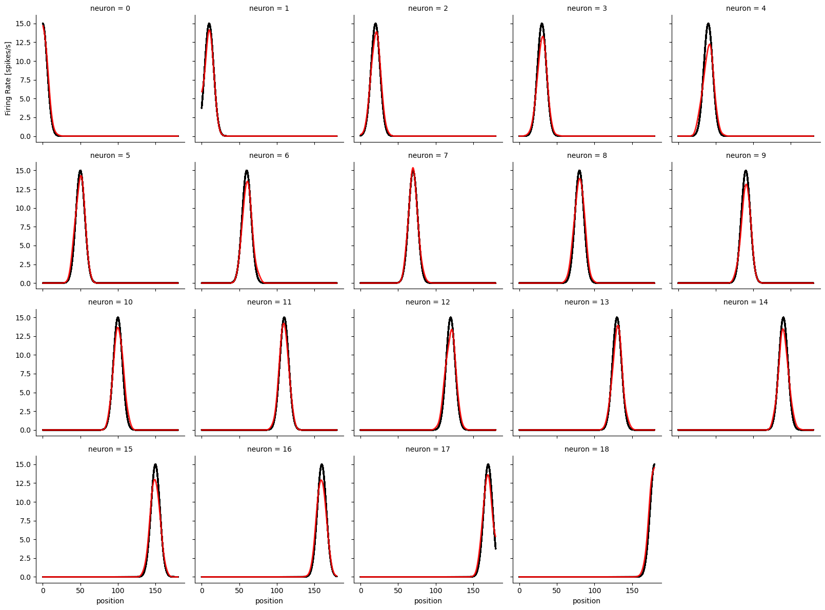
Dimensions without coordinates: neuronAnd plot them versus the true place fields:
g = (decoder.place_fields_ * sampling_frequency).plot(
        x="position", col="neuron", col_wrap=5, color="red", linewidth=2, alpha=0.9, zorder=1, label="Predicted")
g.axes[0, 0].set_ylabel("Firing Rate [spikes/s]")
for ax, place_field in zip(g.axes.flat, place_fields.T):
    ax.plot(position, place_field, linewidth=2, color="black", zorder=-1, label="True")
sns.despine()
We can also plot the state transition model:
fig, ax = plt.subplots(1, 1, figsize=(10, 10))

edge1, edge2 = np.meshgrid(decoder.environment.place_bin_edges_, decoder.environment.place_bin_edges_)
ax.pcolormesh(edge1, edge2, decoder.state_transition_.T, vmin=0.0, vmax=np.percentile(decoder.state_transition_, 99.9))
ax.set_title("Random Walk State Transition Matrix")
ax.set_ylabel("Position at time t-1")
ax.set_xlabel("Position at time t")
ax.axis("square");

Predicting Position#
We can predict the first 50,000 time bins, which produces an labeled array called results:
time_ind = slice(0, 50000)

results = decoder.predict(spikes[time_ind], time=time[time_ind])
results
INFO:replay_trajectory_classification.decoder:Estimating likelihood...
INFO:replay_trajectory_classification.decoder:Estimating causal posterior...
INFO:replay_trajectory_classification.decoder:Estimating acausal posterior...
<xarray.Dataset>
Dimensions:            (time: 50000, position: 342)
Coordinates:
  * time               (time) float64 0.0 0.001 0.002 0.003 ... 50.0 50.0 50.0
  * position           (position) float64 0.2632 0.7895 1.316 ... 179.2 179.7
Data variables:
    likelihood         (time, position) float64 0.9993 0.9992 ... 0.9998 1.0
    causal_posterior   (time, position) float64 0.002929 0.002929 ... 4.314e-171
    acausal_posterior  (time, position) float64 0.046 0.06159 ... 4.314e-171
Attributes:
data_log_likelihood: -726.859881977992results has three main variables:
likelihood – the probablility of spikes given position
causal_posterior: the probability of position given only past spikes
acausal_posterior: the probability of position given all past and future spikes
You’ll probably want to use the acausal_posterior, but we can visualize both the acausal and causal and overlay the true position (magenta dashed line):
fig, axes = plt.subplots(3, 1, sharex=True, constrained_layout=True, figsize=(15, 7))

spike_ind, neuron_ind = np.nonzero(spikes[time_ind])
c = [cmap.colors[ind] for ind in neuron_ind]
axes[0].scatter(time[spike_ind], neuron_ind + 1, c=c, s=0.5, clip_on=False)
axes[0].set_yticks((1, spikes.shape[1]))
axes[0].set_ylabel('Cells')

results.causal_posterior.plot(x="time", y="position", ax=axes[1], cmap="bone_r", vmin=0.0, vmax=0.05, clip_on=False)
axes[1].plot(time[time_ind], position[time_ind], color="magenta", linestyle="--", linewidth=3, clip_on=False)
axes[1].set_xlabel("")
results.acausal_posterior.plot(x="time", y="position", ax=axes[2], cmap="bone_r", vmin=0.0, vmax=0.05, clip_on=False)
axes[2].plot(time[time_ind], position[time_ind], color="magenta", linestyle="--", linewidth=3, clip_on=False)
axes[2].set_xlabel('Time [s]')
sns.despine(offset=5)

From this, we can see, as expected, that the decoded position (given as a probability of position over time) matches the true position well.
Example using Track Graph#
For anything more complicated than a linear track, you will want to use the track graph to specify the correspondence of 1D and 2D position. Here is an example using a circular track.
Simulated Data Setup#
First we generate some data for a circular track. We also make a track graph (See notebooks/tutorial/01-Introduction_and_Data_Format.ipynb for more information on track graph creation)
from replay_trajectory_classification import make_track_graph, plot_track_graph
import matplotlib.pyplot as plt
from scipy.stats import multivariate_normal

angle = np.linspace(-np.pi, np.pi, num=24, endpoint=False)
radius = 30

node_positions = np.stack((radius * np.cos(angle), radius * np.sin(angle)), axis=1)

node_ids = np.arange(node_positions.shape[0])
edges = np.stack((node_ids, np.roll(node_ids, shift=1)), axis=1)

track_graph = make_track_graph(node_positions, edges)

position_angles = np.linspace(-np.pi, 31 * np.pi, num=360_000, endpoint=False)
position = np.stack((radius * np.cos(position_angles), radius * np.sin(position_angles)), axis=1)

fig, ax = plt.subplots(figsize=(10, 10))
plot_track_graph(track_graph, ax=ax)
ax.tick_params(left=True, bottom=True, labelleft=True, labelbottom=True)
ax.set_xlabel("X-Position")
ax.set_ylabel("Y-Position")
ax.spines["top"].set_visible(False)
ax.spines["right"].set_visible(False)

ax.scatter(position[:, 0], position[:, 1], alpha=0.25, s=10, zorder=11, color="magenta")
<matplotlib.collections.PathCollection at 0x7f90bf73c250>

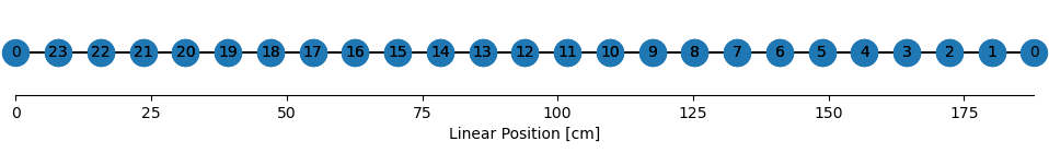
If we want to linearize the track, we need to map the 2D position to 1D position. We do this by sepcifying the edge_order and edge_spacing:
from replay_trajectory_classification import plot_graph_as_1D

edge_spacing = 0
n_nodes = len(track_graph.nodes)
edge_order = np.stack((np.roll(np.arange(n_nodes-1, -1, -1), 1),
                       np.arange(n_nodes-1, -1, -1)), axis=1)

fig, ax = plt.subplots(figsize=(n_nodes // 2, 1))
plot_graph_as_1D(track_graph,
                 edge_spacing=edge_spacing,
                 edge_order=edge_order,
                 ax=ax)
We can use the track_linearization package to linearize the track from 1D to 2D
from track_linearization import get_linearized_position

position_df = get_linearized_position(position, track_graph, edge_order=edge_order, edge_spacing=edge_spacing, use_HMM=False)
position_df
| linear_position | track_segment_id | projected_x_position | projected_y_position | |
|---|---|---|---|---|
| 0 | 0.000000 | 0 | -30.000000 | -3.673940e-15 |
| 1 | 187.949411 | 1 | -29.998916 | -8.235002e-03 |
| 2 | 187.941104 | 1 | -29.997832 | -1.647031e-02 |
| 3 | 187.932798 | 1 | -29.996747 | -2.470591e-02 |
| 4 | 187.924491 | 1 | -29.995663 | -3.294182e-02 |
| ... | ... | ... | ... | ... |
| 359995 | 0.041533 | 0 | -29.994579 | 4.117803e-02 |
| 359996 | 0.033226 | 0 | -29.995663 | 3.294182e-02 |
| 359997 | 0.024919 | 0 | -29.996747 | 2.470591e-02 |
| 359998 | 0.016612 | 0 | -29.997832 | 1.647031e-02 |
| 359999 | 0.008306 | 0 | -29.998916 | 8.235002e-03 |
360000 rows × 4 columns
Now let’s check to see if the linearization looks correct.
plt.figure(figsize=(20, 5))

sampling_frequency = 1000
time = np.arange(position_df.linear_position.size) / sampling_frequency
plt.scatter(time, position_df.linear_position, clip_on=False, s=1, color='magenta')
plt.xlabel('Time')
plt.ylabel('Linear Position')
sns.despine()

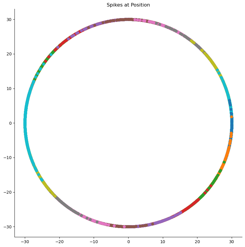
Now let’s simulate neurons with 2D place fields. Here simulate 20 cells with place fields spaced equally around the track.
from replay_trajectory_classification.simulate import simulate_neuron_with_place_field

angle = np.linspace(-np.pi, np.pi, num=20, endpoint=False)

place_field_centers = np.stack((radius * np.cos(angle), radius * np.sin(angle)), axis=1)

spikes = np.stack([simulate_neuron_with_place_field(center, position, sampling_frequency=sampling_frequency, variance=6.0**2)
                   for center in place_field_centers[::-1]], axis=1)

fig, ax = plt.subplots(figsize=(10, 10))
for spike in spikes.T:
    spike_ind = np.nonzero(spike)[0]
    ax.scatter(position[spike_ind, 0], position[spike_ind, 1])

ax.axis("square")
ax.set_title('Spikes at Position')
sns.despine()
Using the track graph with the decoder#
IMPORTANT!!!
In order to get the proper transition matrix and binning of linear position, we need to specify:
track_graphedge_orderedge_spacing
in the environment.
This is the same as the linearization.
from replay_trajectory_classification import SortedSpikesDecoder

environment = Environment(place_bin_size=0.5,
                         track_graph=track_graph,
            edge_order=edge_order,
            edge_spacing=edge_spacing)
transition_type = RandomWalk(movement_var=0.25)

decoder = SortedSpikesDecoder(
    environment=environment,
    transition_type=transition_type,
)

decoder
SortedSpikesDecoder(environment=Environment(environment_name='', place_bin_size=0.5, track_graph=<networkx.classes.graph.Graph object at 0x7f90bf745970>, edge_order=array([[ 0, 23],
       [23, 22],
       [22, 21],
       [21, 20],
       [20, 19],
       [19, 18],
       [18, 17],
       [17, 16],
       [16, 15],
       [15, 14],
       [14, 13],
       [13, 12],
       [12, 11],
       [11, 10],
       [10,  9],
       [ 9,  8],
       [ 8,  7],
       [ 7,  6],
       [ 6,  5],
       [ 5,  4],
       [ 4,  3],
       [ 3,  2],
       [ 2,  1],
       [ 1,  0]]), edge_spaci...l_holes=False, dilate=False),
                    infer_track_interior=True,
                    initial_conditions_type=UniformInitialConditions(),
                    sorted_spikes_algorithm='spiking_likelihood_kde',
                    sorted_spikes_algorithm_params={'block_size': None,
                                                    'position_std': 6.0,
                                                    'use_diffusion': False},
                    transition_type=RandomWalk(environment_name='', movement_var=0.25, movement_mean=0.0, use_diffusion=False))
In a Jupyter environment, please rerun this cell to show the HTML representation or trust the notebook. On GitHub, the HTML representation is unable to render, please try loading this page with nbviewer.org.
SortedSpikesDecoder(environment=Environment(environment_name='', place_bin_size=0.5, track_graph=<networkx.classes.graph.Graph object at 0x7f90bf745970>, edge_order=array([[ 0, 23],
       [23, 22],
       [22, 21],
       [21, 20],
       [20, 19],
       [19, 18],
       [18, 17],
       [17, 16],
       [16, 15],
       [15, 14],
       [14, 13],
       [13, 12],
       [12, 11],
       [11, 10],
       [10,  9],
       [ 9,  8],
       [ 8,  7],
       [ 7,  6],
       [ 6,  5],
       [ 5,  4],
       [ 4,  3],
       [ 3,  2],
       [ 2,  1],
       [ 1,  0]]), edge_spaci...l_holes=False, dilate=False),
                    infer_track_interior=True,
                    initial_conditions_type=UniformInitialConditions(),
                    sorted_spikes_algorithm='spiking_likelihood_kde',
                    sorted_spikes_algorithm_params={'block_size': None,
                                                    'position_std': 6.0,
                                                    'use_diffusion': False},
transition_type=RandomWalk(environment_name='', movement_var=0.25, movement_mean=0.0, use_diffusion=False))decoder.fit(position_df.linear_position,
spikes)
INFO:replay_trajectory_classification.decoder:Fitting initial conditions...
INFO:replay_trajectory_classification.decoder:Fitting state transition...
INFO:replay_trajectory_classification.decoder:Fitting place fields...
SortedSpikesDecoder(environment=Environment(environment_name='', place_bin_size=0.5, track_graph=<networkx.classes.graph.Graph object at 0x7f90bf745970>, edge_order=array([[ 0, 23],
       [23, 22],
       [22, 21],
       [21, 20],
       [20, 19],
       [19, 18],
       [18, 17],
       [17, 16],
       [16, 15],
       [15, 14],
       [14, 13],
       [13, 12],
       [12, 11],
       [11, 10],
       [10,  9],
       [ 9,  8],
       [ 8,  7],
       [ 7,  6],
       [ 6,  5],
       [ 5,  4],
       [ 4,  3],
       [ 3,  2],
       [ 2,  1],
       [ 1,  0]]), edge_spaci...l_holes=False, dilate=False),
                    infer_track_interior=True,
                    initial_conditions_type=UniformInitialConditions(),
                    sorted_spikes_algorithm='spiking_likelihood_kde',
                    sorted_spikes_algorithm_params={'block_size': None,
                                                    'position_std': 6.0,
                                                    'use_diffusion': False},
                    transition_type=RandomWalk(environment_name='', movement_var=0.25, movement_mean=0.0, use_diffusion=False))
In a Jupyter environment, please rerun this cell to show the HTML representation or trust the notebook. On GitHub, the HTML representation is unable to render, please try loading this page with nbviewer.org.
SortedSpikesDecoder(environment=Environment(environment_name='', place_bin_size=0.5, track_graph=<networkx.classes.graph.Graph object at 0x7f90bf745970>, edge_order=array([[ 0, 23],
       [23, 22],
       [22, 21],
       [21, 20],
       [20, 19],
       [19, 18],
       [18, 17],
       [17, 16],
       [16, 15],
       [15, 14],
       [14, 13],
       [13, 12],
       [12, 11],
       [11, 10],
       [10,  9],
       [ 9,  8],
       [ 8,  7],
       [ 7,  6],
       [ 6,  5],
       [ 5,  4],
       [ 4,  3],
       [ 3,  2],
       [ 2,  1],
       [ 1,  0]]), edge_spaci...l_holes=False, dilate=False),
                    infer_track_interior=True,
                    initial_conditions_type=UniformInitialConditions(),
                    sorted_spikes_algorithm='spiking_likelihood_kde',
                    sorted_spikes_algorithm_params={'block_size': None,
                                                    'position_std': 6.0,
                                                    'use_diffusion': False},
                    transition_type=RandomWalk(environment_name='', movement_var=0.25, movement_mean=0.0, use_diffusion=False))
Again we can plot the place fields
fig, ax = plt.subplots(figsize=(10, 3))
(decoder.place_fields_ * sampling_frequency).plot(x="position", hue="neuron", add_legend=False, ax=ax)
ax.set_xlabel('Linear Position')
ax.set_ylabel('Firing Rate')
ax.set_xlim((0, position_df.linear_position.max()))
sns.despine()

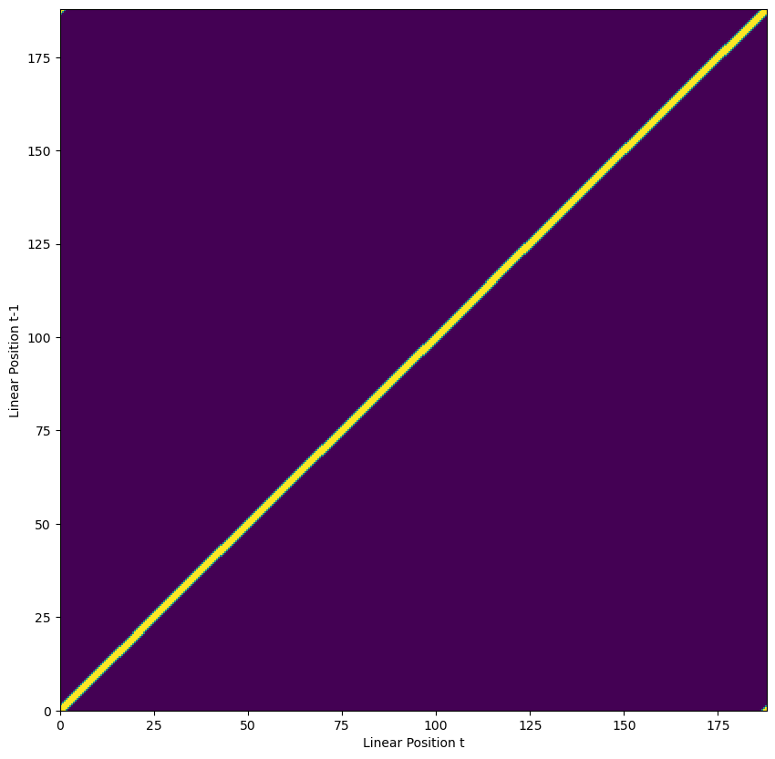
Here is the random walk transition matrix.
Notice that there is now a spot of color at the upper left and bottom right corner of the transition matrix that indicates the position can move between the first and last linear position (which makes sense because this is a circle).
plt.figure(figsize=(10, 10))
bin1, bin2 = np.meshgrid(decoder.environment.place_bin_edges_, decoder.environment.place_bin_edges_)
plt.pcolormesh(bin1, bin2, decoder.state_transition_.T, vmin=0.0, vmax=0.01)
plt.xlabel('Linear Position t')
plt.ylabel('Linear Position t-1');
We can predict the data from the first 50,000 time points as before:
time_ind = slice(0, 50_000)
results = decoder.predict(spikes[time_ind], time=time[time_ind])

results
INFO:replay_trajectory_classification.decoder:Estimating likelihood...
INFO:replay_trajectory_classification.decoder:Estimating causal posterior...
INFO:replay_trajectory_classification.decoder:Estimating acausal posterior...
<xarray.Dataset>
Dimensions:            (time: 50000, position: 384)
Coordinates:
  * time               (time) float64 0.0 0.001 0.002 0.003 ... 50.0 50.0 50.0
  * position           (position) float64 0.2447 0.7342 1.224 ... 187.2 187.7
Data variables:
    likelihood         (time, position) float64 0.9989 0.9988 ... 0.9987 0.9987
    causal_posterior   (time, position) float64 0.002606 0.002606 ... 4.562e-13
    acausal_posterior  (time, position) float64 0.04053 0.03893 ... 4.562e-13
Attributes:
data_log_likelihood: -561.173387422146And we can see that the linear position and decode match
fig, axes = plt.subplots(2, 1, figsize=(15, 5), sharex=True, constrained_layout=True)

spike_time_ind, neuron_ind = np.nonzero(spikes[time_ind])
cmap = plt.get_cmap('tab20')
c = [cmap.colors[ind] for ind in neuron_ind]
axes[0].scatter(time[time_ind][spike_time_ind], neuron_ind, clip_on=False, s=1, c=c)
axes[0].set_ylabel('Cells')

results.acausal_posterior.plot(x="time", y="position", ax=axes[1],
                               robust=True, cmap="bone_r", vmin=0.0, vmax=0.05,
                               clip_on=False)
axes[1].scatter(time[time_ind], position_df.iloc[time_ind].linear_position, color="magenta", s=1, clip_on=False)
axes[1].set_ylabel('Linear Position')
axes[1].set_xlabel('Time')
sns.despine(offset=5)

Decoding in 2D#
environment = Environment(place_bin_size=2.5)
transition_type = RandomWalk(movement_var=0.25)

decoder = SortedSpikesDecoder(
    environment=environment,
    transition_type=transition_type,
    sorted_spikes_algorithm='spiking_likelihood_kde',
    sorted_spikes_algorithm_params={'block_size': None,
                                    'position_std': 3.0},
)

decoder.fit(position, spikes)
INFO:replay_trajectory_classification.decoder:Fitting initial conditions...
INFO:replay_trajectory_classification.decoder:Fitting state transition...
INFO:replay_trajectory_classification.decoder:Fitting place fields...
SortedSpikesDecoder(environment=Environment(environment_name='', place_bin_size=2.5, track_graph=None, edge_order=None, edge_spacing=None, is_track_interior=None, position_range=None, infer_track_interior=True, fill_holes=False, dilate=False),
                    infer_track_interior=True,
                    initial_conditions_type=UniformInitialConditions(),
                    sorted_spikes_algorithm='spiking_likelihood_kde',
                    sorted_spikes_algorithm_params={'block_size': None,
                                                    'position_std': 3.0},
                    transition_type=RandomWalk(environment_name='', movement_var=0.25, movement_mean=0.0, use_diffusion=False))
In a Jupyter environment, please rerun this cell to show the HTML representation or trust the notebook. On GitHub, the HTML representation is unable to render, please try loading this page with nbviewer.org.
SortedSpikesDecoder(environment=Environment(environment_name='', place_bin_size=2.5, track_graph=None, edge_order=None, edge_spacing=None, is_track_interior=None, position_range=None, infer_track_interior=True, fill_holes=False, dilate=False),
                    infer_track_interior=True,
                    initial_conditions_type=UniformInitialConditions(),
                    sorted_spikes_algorithm='spiking_likelihood_kde',
                    sorted_spikes_algorithm_params={'block_size': None,
                                                    'position_std': 3.0},
                    transition_type=RandomWalk(environment_name='', movement_var=0.25, movement_mean=0.0, use_diffusion=False))
time_ind = slice(0, 50_000)
results = decoder.predict(spikes[time_ind], time=time[time_ind])
results
INFO:replay_trajectory_classification.decoder:Estimating likelihood...
INFO:replay_trajectory_classification.decoder:Estimating causal posterior...
INFO:replay_trajectory_classification.decoder:Estimating acausal posterior...
<xarray.Dataset>
Dimensions:            (time: 50000, x_position: 26, y_position: 26)
Coordinates:
  * time               (time) float64 0.0 0.001 0.002 0.003 ... 50.0 50.0 50.0
  * x_position         (x_position) float64 -31.25 -28.75 -26.25 ... 28.75 31.25
  * y_position         (y_position) float64 -31.25 -28.75 -26.25 ... 28.75 31.25
Data variables:
    likelihood         (time, x_position, y_position) float64 nan nan ... nan
    causal_posterior   (time, x_position, y_position) float64 nan nan ... nan
    acausal_posterior  (time, x_position, y_position) float64 nan nan ... nan
Attributes: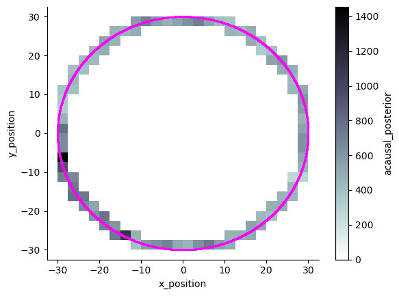
data_log_likelihood: -1822.0986324353144Here is the sum of the probability of 2D decoded positions overlayed with the true position
results.acausal_posterior.sum('time').plot(x='x_position', y='y_position', cmap='bone_r')
plt.scatter(position[time_ind, 0], position[time_ind, 1], color='magenta', s=1, clip_on=False, label='True Position')
sns.despine()
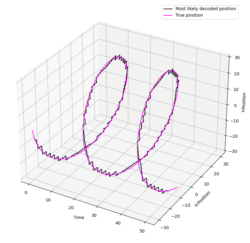
Here is the most likely position over time compared with the true position
map_estimate = results.acausal_posterior.stack(position=['x_position', 'y_position'])
map_estimate = map_estimate.position[map_estimate.argmax('position')]
map_estimate = np.asarray(map_estimate.values.tolist())

plt.figure(figsize=(10, 10))
ax = plt.axes(projection='3d')
ax.plot3D(results.time, map_estimate[:, 0], map_estimate[:, 1], 'black', label='Most likely decoded position')
ax.set_xlabel('Time')
ax.set_ylabel('X-Position')
ax.set_zlabel('Y-Position')

ax.plot3D(results.time, position[time_ind, 0], position[time_ind, 1], 'magenta', label='True position')
ax.set_xlabel('Time')
ax.set_ylabel('X-Position')
ax.set_zlabel('Y-Position')
plt.legend()
<matplotlib.legend.Legend at 0x7f90d1f2b070>